Comparing Similarities and Distance
George G. Vega Yon
2020-03-13
comparing-similarities.RmdPowerset of 3
# Computing
all_raw03 <- similarity(powerset03, statistic = unlist(statistics$alias))
all03 <- all_raw03
all03[!is.finite(all03)] <- NA

all_cor03 <- all03
all_cor03[,statistics$distance] <- -all_cor03[,statistics$distance]
all_cor03 <- cor(all_cor03[,-c(1,2)], use = "pairwise.complete.obs")
# knitr::kable(all_cor, digits = 2)
res <- cbind(a=rownames(all_cor03), as.data.frame(all_cor03))
res <- lapply(2:ncol(res), function(i) {
data.frame(
a = res[,1],
b = colnames(res)[i],
corr = res[,i],
stringsAsFactors = FALSE
)
}) %>%
do.call("rbind", .)
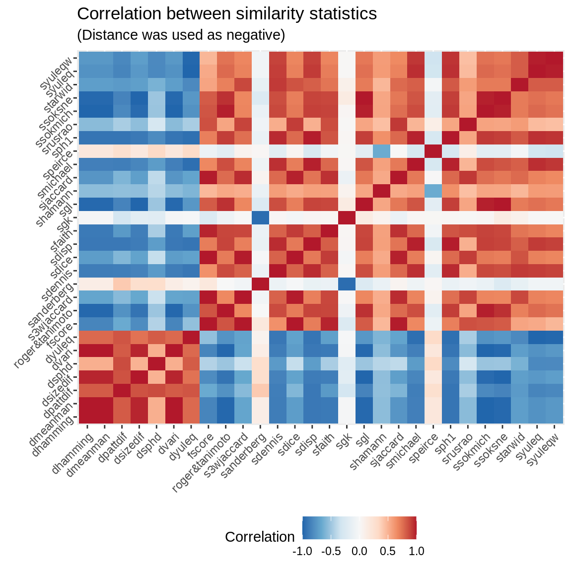
ggplot(res, aes(x=a, y=b, fill=corr))+
scale_fill_distiller(palette = "RdBu") +
geom_bin2d() +
labs(fill = "Correlation") +
labs(title = "Correlation between similarity statistics") +
labs(subtitle = "(Distance was used as negative)") +
theme(
axis.text = element_text(angle = 45, hjust = 1),
legend.position = "bottom",
axis.title = element_blank()
)
lapply(3:ncol(all03), function(i) {

  ans <- data.frame(
    Statistic = colnames(all03)[i],
    `% Miss`    = sum(!is.finite(all03[,i]))/length(all03[,i])*100,
    `Variance`  = var(all03[,i], na.rm=TRUE),
    `Min`       = min(all03[,i], na.rm=TRUE),
    `Max`       = max(all03[,i], na.rm=TRUE),
    `p25`       = quantile(all03[,i], .25, na.rm=TRUE),
    `p75`       = quantile(all03[,i], .75, na.rm=TRUE),
    check.names = FALSE
  )

  ans$IQR <- with(ans, p75 - p25)
  ans

}) %>%
  do.call(rbind, .) %>%
knitr::kable(digits=2)| Statistic | % Miss | Variance | Min | Max | p25 | p75 | IQR | |
|---|---|---|---|---|---|---|---|---|
| 25% | sjaccard | 0.00 | 0.05 | 0.00 | 0.83 | 0.20 | 0.50 | 0.30 |
| 25%1 | sdice | 0.00 | 0.07 | 0.00 | 0.91 | 0.33 | 0.67 | 0.33 |
| 25%2 | s3wjaccard | 0.00 | 0.08 | 0.00 | 0.94 | 0.43 | 0.75 | 0.32 |
| 25%3 | ssokmich | 0.00 | 0.04 | 0.00 | 0.83 | 0.33 | 0.67 | 0.33 |
| 25%4 | ssoksne | 0.00 | 0.04 | 0.00 | 0.91 | 0.50 | 0.80 | 0.30 |
| 25%5 | roger&tanimoto | 0.00 | 0.03 | 0.00 | 0.71 | 0.20 | 0.50 | 0.30 |
| 25%6 | sfaith | 0.00 | 0.03 | 0.00 | 0.83 | 0.25 | 0.50 | 0.25 |
| 25%7 | sgl | 0.00 | 0.04 | 0.00 | 0.91 | 0.50 | 0.80 | 0.30 |
| 25%8 | srusrao | 0.00 | 0.03 | 0.00 | 0.83 | 0.17 | 0.33 | 0.17 |
| 25%9 | dvari | 0.00 | 3.10 | 1.50 | 9.00 | 3.00 | 6.00 | 3.00 |
| 25%10 | dsizedif | 0.00 | 0.04 | 0.03 | 1.00 | 0.11 | 0.44 | 0.33 |
| 25%11 | dsphd | 0.00 | 0.02 | -0.50 | 0.50 | 0.06 | 0.22 | 0.17 |
| 25%12 | dpattdif | 0.00 | 0.04 | 0.00 | 1.00 | 0.00 | 0.33 | 0.33 |
| 25%13 | starwid | 3.12 | 0.09 | -1.00 | 0.20 | -0.45 | -0.20 | 0.25 |
| 25%14 | sph1 | 6.20 | 0.19 | -1.00 | 0.71 | -0.33 | 0.33 | 0.67 |
| 25%15 | dhamming | 0.00 | 0.04 | 0.17 | 1.00 | 0.33 | 0.67 | 0.33 |
| 25%16 | dmeanman | 0.00 | 0.04 | 0.17 | 1.00 | 0.33 | 0.67 | 0.33 |
| 25%17 | sdennis | 3.12 | 0.54 | -1.73 | 1.63 | -0.58 | 0.58 | 1.15 |
| 25%18 | syuleq | 6.20 | 0.65 | -1.00 | 1.00 | -1.00 | 1.00 | 2.00 |
| 25%19 | syuleqw | 6.20 | 0.61 | -1.00 | 1.00 | -1.00 | 1.00 | 2.00 |
| 25%20 | dyuleq | 6.20 | 0.65 | 0.00 | 2.00 | 0.00 | 2.00 | 2.00 |
| 25%21 | smichael | 0.00 | 0.31 | -1.00 | 0.92 | -0.60 | 0.44 | 1.04 |
| 25%22 | sdisp | 0.00 | 0.01 | -0.25 | 0.17 | -0.08 | 0.06 | 0.14 |
| 25%23 | shamann | 0.00 | 0.11 | -1.00 | 1.00 | 0.33 | 0.67 | 0.33 |
| 25%24 | sgk | 9.42 | 1.01 | -3.00 | 0.00 | -0.50 | 0.00 | 0.50 |
| 25%25 | sanderberg | 0.00 | 0.04 | 0.00 | 1.00 | 0.00 | 0.17 | 0.17 |
| 25%26 | speirce | 5.95 | 0.08 | 0.00 | 1.00 | 0.25 | 0.60 | 0.35 |
| 25%27 | fscore | 18.06 | 0.03 | 0.29 | 0.91 | 0.40 | 0.67 | 0.27 |
Of all the measurements shown here, only 6 were defined for all cases. In the case of Anderberg, it might not be the best option because of its negatively correlatedness with most of the measures. Both Jaccard and Hamming, even though popular, show very low variances overall compare to Michael and Hamann, which if you care about heterogeneity in the measurements (this could be a key factor in regression analysis) can be important.